
Assuming functions for life expectancy
If we think about it, no one is safe from sudden death, stroke or even an accident. Such aspects can take us out of the world without the chance to leave any message to those who remain.
In the Western context, death seems to be something dark, a subject to be avoided and feared, we do not talk about it with children and that is why we arrived at a kind of mystification on the subject. But by thinking in the form of time intervals, it is possible to give anyone a correct guess as to how much life he has left. Apart from biblical characters, we can assume that human beings do not live more than 125 years, so it is correct to say that any person alive will still be alive for at most:
[125 – (current age)] years;
in my case, I have no more than 97 years to live.
In a somewhat “cold” way, if a 25 year old asks when he will die, the answer would be “between today and 100 years from now”. Or a 100 year old person asks when he will die, the answer would be “between today and 25 years from now”. But we can reduce this margin of accuracy a little by taking a data from the IBGE (Instituto Brasileiro de Geografia e Estatistica – Brazilian Institute of Geography and Statistics) for 2018, which states the life expectancy of Brazilians is approximately 76,3 years.
Thus, when a child is born (if we assume that life expectancy will remain unchanged long enough) we can determine from the area of that curve, how likely it is to reach each age. With this information in hand and knowing the life expectancy, we could say that this newborn has a 50% chance of passing 76,3 years. Or by complementing this statement, a 50% chance of dying before this same age.
With this single information, if we assume that the life curve is distributed in a linear fashion, we can determine the following probability plot to reach each age:
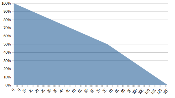
Horizontal axis represents ages and vertical the probability of reaching each one (assuming the distribution is linear).
In the case of this distribution, taking my own age as an example (28 years in the case), we can say that the chance of not having reached that age (dying before 28 years old) would be 18,4%. On the other hand, given that I am 28 years old, the chance within this distribution that I will pass the life expectancy of the Brazilian (76,3 years) is 68,4%. Note that this is calculated in a similar way to that of the newborn (50% chance, plus the fact that 18.4% of that life has already passed).
With this same information, let’s assume that the distribution is not linear, but parabolic, in which case we can determine the following probability graph to reach each age:
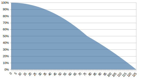
Horizontal axis represents ages and vertical the probability of reaching each one (assuming the distribution is parabolic).
In the case of this distribution, taking my own age as an example (28 years in the case), we can say that the chance of not reaching that age (dying before 28 years old) would be 6,7%. On the other hand, given that I am 28 years old, the chance within this distribution that I will pass the life expectancy of the Brazilian (76,3 years) is 56,7%. Note that this is calculated in a similar way to that of the newborn (50% chance, plus the fact that it has already covered 6,7% of that life).
With this same information, let’s assume that the distribution is not linear, but cubic, in which case we can determine the following probability plot to reach each age:
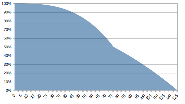
Horizontal axis represents ages and vertical the probability of reaching each one (assuming the distribution is cubic).
In the case of this distribution, taking my own age as an example (28 years in the case), we can say that the chance of not reaching that age (dying before the age of 28) would be 2,5%. On the other hand, given that I am 28 years old, the chance within this distribution that I will pass the life expectancy of the Brazilian (76,3 years) is 52,5%. Note that this is calculated in a similar way to that of the newborn (50% chance, plus the fact that it has already covered 2,5% of that life).
The purpose of this discussion is to highlight the importance of adjusting curves for probability distribution. Because with the information about its beginning (0 years), end (125 years) and average (76,3 years). We can vary this distribution by assuming several functions, such as linear, parabolic, cubic and others that serve this purpose. Note that in the three charts and their respective calculations, we do not add or remove any of the three original information (minimum, maximum and average age). We just changed an assumption of how it behaves in this interval, and so we got three very different results.